What we are really interested in is the detailed mass balance of carbon between the
atmosphere and the earth's surface. The surface can be either land or water, it doesn't matter for argument's sake.
We know that the carbon-cycle between the atmosphere and the biota is relatively fast and the majority of the exchange has a turnover of just a few years. Yet, what we are really interested in is the deep exchange of the carbon with slow-releasing stores. This process is described by diffusion and that is where we can use the Fokker-Planck to represent the flow of CO2.
This part can't be debated because this is the way that the flow of all particles works; they call it the master equation because it invokes the laws of probability and in particular the basic random walk that just about every physical phenomenon displays.
The origin of the master model is best described by considering a flow graph and
drawing edges between compartments of the system. This is often referred to as a
compartment or box model. The flows go both ways and are random, and thus model the random walk between compartments.
The following chart is a Markov model consisting of 50 stages of deeper sequestering with each slab having a constant but small hop rate. The single interface between the atmosphere and the earth has a faster hopping rate corresponding to faster carbon cycling.
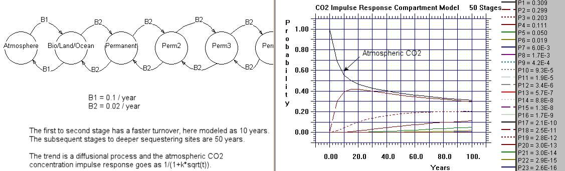
That shows how you would solve the system numerically. The basic analytical
solution to the Fokker-Planck assuming a planar source and one-dimensional diffusion is the following:
$$ \frac1{\sqrt{2 \pi t}} exp(-x^2/{2t}) $$
Consider that x=0 near the surface, or at the atmosphere/earth interface.
Because of that, this expression can be approximated by
$$ n(t)=\frac{q}{\sqrt{t}} $$
where n(t) is the concentration evolution over time and q is a scaling factor for
that concentration.
First thing one notices about this expression is that n(t) has a fat tail and
after a rapid initial fall-off only slowly decreases over time. The physical meaning is that, due to diffusion, the concentration randomly walks between the interface and deeper locations in the earth. The square root of time dependence is a classic trait of all random walks and you can't escape seeing this if you have ever watched nature in action. That is just the way particles move around.
For CO2 concentration this in fact describes the evolution of the adjustment
time, and it accurately reflects the infamous IPCC curve for the atmospheric CO2 impulse response. It is called an impulse response because that is the response that one would expect based on an initial impulse of CO2 concentration.
But that is just the first part of the story. As an impulse response, n(t) describes what is called a single point source of initial concentration and its slow evolution. In practice, fossil-fuel emissions generate a continuous stream of CO2 impulses. These have to be incorporated somehow. The way this is done is by the mathematical technique called convolution.
So consider that the incoming stream of new CO2 from fossil fuel emissions is
called F(t). This becomes the forcing function.
Then the system evolution is described by the equation
$$ c(t)=n(t)*F(t) $$
where the operator * is not a multiplication but signifies convolution.
Again, there is no debate over the fundamental correctness of what has been said
so far. This is exactly the way a system will respond.
If we are now to put this into practice and see how well it describes the actual
evolution of CO2, we can understand ever nagging issue that has haunted skeptical observers. It really all becomes very clear.
For the forcing function F(t) we use a growing power law.
$$ F(t) = k t^N $$
where N is the power and k is a scaling constant.
This roughly represents the atmospheric emissions through the industrial era if
we use a power law of N=4. See the following curve:

So all we really want to solve is the convolution of n(t) with F(t). By using
Laplace transforms on the convolution expression, the answer comes out
surprisingly clean and concise. Ignoring the scaling factor :
$$ c(t) \sim t^{N+1/2} $$
With that solved, we can now answer the issue of where the "missing" CO2 went
to. This is an elementary problem of integrating the forcing function, F(t), over time and then comparing the concentration, c(t), to this value. Then this ratio of c(t) to the integral of F(t) is the amount of CO2 that remains in the atmosphere.
Working out the details, this ratio is:
$$ q \sqrt{\frac{\pi}{t}}\frac{(N+1)!}{(N+0.5)!} $$
Plugging in numbers for this expression, q=1, and N=4, then the ratio is about 0.
28 after 200 years of growth. This means that 0.72 of the CO2 is going back into
the deep-stores of the carbon cycle, and 0.28 is remaining in the atmosphere.
If we choose a value of q=2, then 0.56 remains in the atmosphere and 0.44 goes
into the deep store. This ratio is essentially related to the effective
diffusion coefficient of the carbon going into the deep store.
Come up with a good number for the diffusion coefficient and we have an explanation of the evolution of the "missing carbon".
BTW, This is useful for modifying the numbers.
alpha equation
Alexander Harvey comment
R(t,0) = α/Sqrt(t) where α can be derived from the diffusivity and thermal capacity.
The general case R(t,λ) is not easily stated but can be calculated by the deconvolution of R(t,0) with the unit impulse fucntion to which an impulse term 1/λ at t=0 is added and the whole is deconvoluted with the unit impulse function. This is I think the same as can be achieved using the Laplace transforms in the continuous case.
This comment is the closest to my own thinking on the topic. The 1/Sqrt(t) profile is likely the explanation for the "fat-tail" in the residence cum adjustment time that the IPCC has been publishing. Consider this (EVALUATING THE SOCIAL COSTS OF GREENHOUSE GAS)
To represent this carbon cycle, Maier-Reimer and Hasselmann (1987) have suggested that the carbon stock be represented as a series of five boxes, each with a constant, but different atmospheric lifetime. That is, each box is modelled as in equation (7), and atmospheric concentration is a weighted sum of all five boxes. Maier-Reimer and Hasselmann suggested lifetimes of 1.9 years, 17.3 years, 73.6 years, 362.9 years and infinity, to which they attach weights of 0.1, 0.25, 0.32, 0.2 and 0.13, respectivelyI punched these numbers in and this is what it looks like in comparison to a disordered diffusion profile:

The boxes they talk about simply describes a model of maximum entropy disorder. If the maximum entropy disorder is governed by force (i.e. drift), the profile will go toward 1/(1+t/a) and if it is governed by diffusion (i.e. random walk) it will go as 1/(1+sqrt(t/a)). Selecting a weighted sum of exponential lifetimes is exactly the same as choosing a maximum entropy distribution of rates, and I believe that whatever their underlying simulation is that it will asymptotically trend toward this result. The lifetime they choose for infinity is needed because otherwise the fat-tail will eventually disappear.
This is the MaxEnt derivation
integral exp(-1/(x*t))*exp(-x)/sqrt(x*t)*dx from x=0 to x=infinity

No comments:
Post a Comment